Programming with R: Challenges

Introduction to RStudio

Challenge 1

Which of the following are valid R variable names?

min_height
max.height
_age
.mass
MaxLength
min-length
2widths
celsius2kelvin

Solution to challenge 1

The following can be used as R variables:

min_height
max.height
MaxLength
celsius2kelvin

The following creates a hidden variable:

.mass

The following will not be able to be used to create a variable

_age
min-length
2widths

Challenge 2

What will be the value of each variable after each statement in the following program?

mass <- 47.5
age <- 122
mass <- mass * 2.3
age <- age - 20

Solution to challenge 2

mass <- 47.5

This will give a value of 47.5 for the variable mass.

age <- 122

This will give a value of 122 for the variable age.

mass <- mass * 2.3

This will multiply the existing value of 47.5 by 2.3 to give a new value of 109.25 to the variable mass.

age <- age - 20

This will subtract 20 from the existing value of 122 to give a new value of 102 to the variable age.

Challenge 3

Run the code from the previous challenge, and write a command to compare mass to age. Is mass larger than age?

Solution to challenge 3

One way of answering this question in R is to use the > to set up the following:

mass > age

[1] TRUE

This should yield a boolean value of TRUE since 109.25 is greater than 102.

Challenge 4

Install the packages ggplot2 and dplyr

After installing, load both of these packages so they are active. Try using both ways that we discussed.

(Note: We will be using these packages in future lessons, so ask a helper for assistance if you have difficulties)

Solution to challenge 5

We can use the install.packages command to install the required packages.

install.packages("ggplot2")
install.packages("dplyr")

You can also install packages through the Packages tab in the lower right pane of RStudio by clicking Install and then typing in the names of the packages we want to install.

To load the packages use the following commands:

library(ggplot2)
library(dplyr)

Or you can click the corresponding checkbox next to the name of the package from the list in the Packages tab.

Seeking Help

Challenge 1

Look at the help for the c function. Try the following commands and see if you can use the help file to explain the output you see:

c(1, 2, 3)
c('d', 'e', 'f')
c(1, 5, 'g')

Solution to Challenge 1

c(1,2,3)
[1] 1 2 3
c('d','e','f')
[1] "d" "e" "f"
c(1,5,'g')
[1] "1" "5" "g"

The c function creates a vector, which is a sequence of individual elements in R. In a vector, all elements must be the same data type. In the first case, we created a numeric vector. For the second, our vector is a character vector which you can see by the quotes that R put around each element. In the third example, since we gave R both numeric and character elements, R converted all the elements to characters so that our vector contained all the same type of elements.

Don’t worry if this is confusing right now. We will clarify more in our next lesson about data structures in R.

Challenge 2

Look at the help for the typeof function. What does this function do? Try creating the following objects and using this function on them.

1. m <- 15
2. n <- “Lincoln”

Explain to your neighbor what this function is telling us about these objects:

Solution to Challenge 2

help("typeof")
?typeof

We can see from the help file that typeof tells us the type of an object in R. We will discuss R data types further in the next lecture.

m <- 15
typeof(m)

[1] "double"

This is telling us that m is the data type double which is a numeric data type in R.

n <- "Lincoln"
typeof(n)

[1] "character"

Here, n is the data type character which is the data type R uses for strings.

Challenge 3 - Advanced

The read.table function is used to read data from external files into the R environment. For example: to read in a file called “data.csv” you would use the following command:

read.table(file = "data.csv")

Look at the help for the read.table function.

What argument would you use if you wanted to read in a file without a header? What argument would allow you to switch between a comma separated file and a tab separated file?

Solution to Challenge 3

To view the help for the read.table function, you can type one of the following commands into your console:

help("read.table")
?read.table

By looking at the arguments section of the help file, we can see that to prevent R from automatically assuming the first row of your file is a header row, you would specify header = FALSE.

read.table(file = "data.csv", header = FALSE)

To switch between comma separated files (csv) and tab separated files (tsv), you would use the sep argument.

Data Structures

Challenge 1

Predict what will happen if we perform an operation between two vectors of different size?

Test your guess by creating two vectors of different lengths using the colon operator and adding or multiplying them together.

Solution to Challenge 1

a <- 1:10
b <- 1:5
a * b

[1]  1  4  9 16 25  6 14 24 36 50

Notice how R repeated the shorter vector until it had finished operating on every element of the larger vector. This is known as “vector recycling”.

If your shorter vector is not a even multiple of the larger one, R will still perform the operation but it will give you the following error message:

Warning message:
In a * b : longer object length is not a multiple of shorter object length

Challenge 2

What happens when we create a vector that combines data types?

Try creating a vector named my_vector containing the elements 1, “four”, and TRUE. What does the vector look like?

Use the str command to determine what data type is in your vector?

Solution to Challenge 2

my_vector <- c(1, "four", TRUE)
my_vector

[1] "1"    "four" "TRUE"

str(my_vector)

 chr [1:3] "1" "four" "TRUE"

See the quotes around each element of my_vector? R turned every element of the vector into a character. Since all elements of the vector must be of the same data type, R picked the best one based on the data we gave it. This is called type coercion. Type coercion can cause problems if your data is not consistant or if it is assigned to an unexpected data type, so we need to watch for it as we work with data in R.

We can manually coerce the data by using commands such as as.numeric or as.character. For more information on how these commands work, you can read their help documentation by typing ?as.numeric or ?as.character.

Challenge 3

R also vectorizes functions on character vectors as well.

Use the c function to create a character vector named colors with the values: “red”, “yellow” and “blue”. Use the paste function to combine "My ball is" with each element of your vector.

Solution to Challenge 2

colors <- c("red", "yellow", "blue")
paste("My ball is", colors)

[1] "My ball is red"    "My ball is yellow"
[3] "My ball is blue"  

Subsetting Data

Challenge 1

Given the following code:

x <- c(5.4, 6.2, 7.1, 4.8, 7.5)
names(x) <- c('a', 'b', 'c', 'd', 'e')
print(x)

  a   b   c   d   e 
5.4 6.2 7.1 4.8 7.5 

Come up with at least 3 different commands that will produce the following output:

  b   c   d 
6.2 7.1 4.8 

After you find 3 different commands, compare notes with your neighbour. Did you have different strategies?

Solution to Challenge 1

x[2:4]

  b   c   d 
6.2 7.1 4.8 

x[-c(1,5)]

  b   c   d 
6.2 7.1 4.8 

x[c("b", "c", "d")]

  b   c   d 
6.2 7.1 4.8 

x[c(2,3,4)]

  b   c   d 
6.2 7.1 4.8 

Challenge 2

Run the following code to define vector x as above:

x <- c(5.4, 6.2, 7.1, 4.8, 7.5)
names(x) <- c('a', 'b', 'c', 'd', 'e')
print(x)

  a   b   c   d   e 
5.4 6.2 7.1 4.8 7.5 

Given this vector x, what would you expect the following to do?

x[-which(names(x) == "g")]

Try out this command and see what you get. Did this match your expectation? Why did we get this result? (Tip: test out each part of the command on it’s own - this is a useful debugging strategy)

Solution to Challenge 2

The which command returns the index of every TRUE value in its input. The names(x) == "g" command didn’t return any TRUE values. Because there were no TRUE values passed to the which command, it returned an empty vector. Negating this vector with the minus sign didn’t change its meaning. Because we used this empty vector to retrieve values from x, it produced an empty numeric vector. It was a named numeric empty vector because the vector type of x is “named numeric” since we assigned names to the values (try str(x) ).

Challenge 3

While it is not recommended, it is possible for multiple elements in a vector to have the same name. Consider this examples:

y <- 1:3
y

[1] 1 2 3

names(y) <- c('a', 'a', 'a')
y

a a a 
1 2 3 

Can you come up with a command that will only return one of the ‘a’ values and a different command that will return all of the ‘a’ values? Does your answer differ from your neighbors?

Solution to challenge 3

y['a']  # only returns first value

a 
1 

y[which(names(y) == 'a')]  # returns all three values

a a a 
1 2 3 

Challenge 4

Given the following code:

x <- c(5.4, 6.2, 7.1, 4.8, 7.5)
names(x) <- c('a', 'b', 'c', 'd', 'e')
print(x)

  a   b   c   d   e 
5.4 6.2 7.1 4.8 7.5 

Write a subsetting command to return the values in x that are greater than 4 and less than 7.

Solution to Challenge 4

x_subset <- x[x<7 & x>4]
print(x_subset)

  a   b   d 
5.4 6.2 4.8 

Exploring Data Frames

Challenge 1

There are several subtly different ways to call variables, observations and elements from data.frames:

• cats[1]
• cats$coat
• cats[“coat”]
• cats[1, 1]
• cats[, 1]
• cats[1, ]

Try out these examples and explain what is returned by each one.

Hint: Use the function typeof to examine what is returned in each case.

Solution to Challenge 1

cats[1]

    coat
1 calico
2  black
3  tabby

We can think of a data frame as a list of vectors. The single brace [1] returns the first slice of the list, as another list. In this case it is the first column of the data frame.

cats$coat

[1] calico black  tabby 
Levels: black calico tabby

This example uses the $ character to address items by name. coat is the first column of the data frame, again a vector of type factor.

cats["coat"]

    coat
1 calico
2  black
3  tabby

Here we are using a single brace ["coat"] replacing the index number with the column name. Like example 1, the returned object is a list.

cats[1, 1]

[1] calico
Levels: black calico tabby

This example uses a single brace, but this time we provide row and column coordinates. The returned object is the value in row 1, column 1. The object is an integer but because it is part of a vector of type factor, R displays the label “calico” associated with the integer value.

cats[, 1]

[1] calico black  tabby 
Levels: black calico tabby

Like the previous example we use single braces and provide row and column coordinates. The row coordinate is not specified, R interprets this missing value as all the elements in this column vector.

cats[1, ]

    coat weight likes_string
1 calico    2.1         TRUE

Again we use the single brace with row and column coordinates. The column coordinate is not specified. The return value is a list containing all the values in the first row.

Challenge 2

Remember that you can create a new data.frame right from within R with the following syntax:

df <- data.frame(id = c('a', 'b', 'c'),
                 x = 1:3,
                 y = c(TRUE, TRUE, FALSE),
                 stringsAsFactors = FALSE)

Note that the stringsAsFactors setting allows us to tell R that we want to preserve our character fields and not have R convert them to factors.

Make a data.frame that holds the following information for yourself:

• first name
• last name
• lucky number

Then use rbind to add an entry for the people sitting beside you. Finally, use cbind to add a column with each person’s answer to the question, “Is it time for coffee break?”

Solution to Challenge 2

df <- data.frame(first = c('Grace'),
                 last = c('Hopper'),
                 lucky_number = c(0),
                 stringsAsFactors = FALSE)
df <- rbind(df, list('Marie', 'Curie', 238) )
df <- cbind(df, coffeetime = c(TRUE,TRUE))

Challenge 3

Read the output of str(gapminder) again; this time, use what you’ve learned about R’s basic data types, factors, and vectors, as well as the output of functions like colnames and dim to explain what everything that str prints out for gapminder means.

Can you determine what data each column holds? Do the data types make sense for these types of data? If not, what data type would you recommend?

If there are any parts you can’t interpret, discuss with your neighbors!

Solution to Challenge 3

The object gapminder is a data frame with 1704 entries and 6 columns.

The 6 columns contain the following data and types:

• country: a factor with 142 levels - The country of which the rest of the data in the row is for.
• continent: a factor with 5 levels - The continent in which the target country is located.
• year: integer vector - The year for which the data was obtained
• pop: integer vector - The total population in the target country for the target year.
• lifeExp: numeric vector - The average life expectancy for the target country during the target year.
• gdpPercap: numeric vector - The average GDP per capita for the target country during the target year.

Challenge 4

Fix each of the following common data frame subsetting errors:

1. Extract observations collected for the year 1957

   gapminder[gapminder$year = 1957,]
   

2. Extract all columns except 1 through to 4

   gapminder[,-1:4]
   

3. Extract the rows where the life expectancy is longer the 80 years

   gapminder[gapminder$lifeExp > 80]
   

4. Extract the first row, and the fourth and fifth columns (lifeExp and gdpPercap).

   gapminder[1, 4, 5]
   

5. Advanced: extract rows that contain information for the years 2002 and 2007

   gapminder[gapminder$year == 2002 | 2007,]
   

Solution to Challenge 4

Fix each of the following common data frame subsetting errors:

1. Extract observations collected for the year 1957

   # gapminder[gapminder$year = 1957,]
   gapminder[gapminder$year == 1957,]
   

2. Extract all columns except 1 through to 4

   # gapminder[,-1:4]
   gapminder[,-c(1:4)]
   

3. Extract the rows where the life expectancy is longer the 80 years

   # gapminder[gapminder$lifeExp > 80]
   gapminder[gapminder$lifeExp > 80,]
   

4. Extract the first row, and the fourth and fifth columns (lifeExp and gdpPercap).

   # gapminder[1, 4, 5]
   gapminder[1, c(4, 5)]
   

5. Advanced: extract rows that contain information for the years 2002 and 2007

    # gapminder[gapminder$year == 2002 | 2007,]
    gapminder[gapminder$year == 2002 | gapminder$year == 2007,]
    gapminder[gapminder$year %in% c(2002, 2007),]
   

Challenge 5

1. Why does gapminder[1:20] return an error? How does it differ from gapminder[1:20, ]?

2. Create a new data.frame called gapminder_small that only contains rows 1 through 9 and 19 through 23. You can do this in one or two steps.

Solution to Challenge 5

1. gapminder is a data.frame so needs to be subsetted on two dimensions. gapminder[1:20, ] subsets the data to give the first 20 rows and all columns.

2. There are several different ways to accomplish this task:

First, you can do it in two steps by subsetting all the rows 1 through 23, then removing rows 10 through 18:

gapminder_small <- gapminder[1:23, ]
gapminder_small <- gapminder_small[-18:-10, ]

Or, you can first subset rows 1 through 9, then use rbind to concatenate the next subset of rows 10 through 18:

gapminder_small <- gapminder[1:9, ]
gapminder_small <- rbind(gapminder_small, gapminder[19:23, ]

Or you can do this in a single step by combining your ranges:

gapminder_small <- gapminder[c(1:9, 19:23), ]

There are probably other ways to accomplish this task. Did you come up with any that we didn’t show here?

Control Flow

Challenge 1

Use an if statement to print a suitable message reporting whether there are any records from 2002 in the gapminder dataset. Now do the same for 2012.

Solution to Challenge 1

We will first see a solution to Challenge 1 which does not use the any function. We first obtain a logical vector describing which element of gapminder$year is equal to 2002:

gapminder[(gapminder$year == 2002),]

Then, we count the number of rows of the data.frame gapminder that correspond to the 2002:

rows2002_number <- nrow(gapminder[(gapminder$year == 2002),])

The presence of any record for the year 2002 is equivalent to the request that rows2002_number is one or more:

rows2002_number >= 1

Putting all together, we obtain:

if(nrow(gapminder[(gapminder$year == 2002),]) >= 1){
   print("Record(s) for the year 2002 found.")
}

All this can be done more quickly with any. The logical condition can be expressed as:

if(any(gapminder$year == 2002)){
   print("Record(s) for the year 2002 found.")
}

Challenge 2

Compare the objects output_vector and output_vector2. Are they the same? If not, why not? How would you change the last block of code to make output_vector2 the same as output_vector?

Solution to Challenge 2

We can check whether the two vectors are identical using the all function:

all(output_vector == output_vector2)

However, all the elements of output_vector can be found in output_vector2:

all(output_vector %in% output_vector2)

and vice versa:

all(output_vector2 %in% output_vector)

therefore, the element in output_vector and output_vector2 are just sorted in a different order. This is because as.vector outputs the elements of an input matrix going over its column. Taking a look at output_matrix, we can notice that we want its elements by rows. The solution is to transpose the output_matrix. We can do it either by calling the transpose function t or by inputing the elements in the right order. The first solution requires to change the original

output_vector2 <- as.vector(output_matrix)

into

output_vector2 <- as.vector(t(output_matrix))

The second solution requires to change

output_matrix[i, j] <- temp_output

into

output_matrix[j, i] <- temp_output

Challenge 3

Use the following commands to create two vectors each containing 5 random values:

rows <- rpois(5, lambda=5)
cols <- rpois(5, lambda=5)

Modify our previous for loops to now fill our 5 x 5 matrix with the product of the respective values in rows and cols. (ie position [2, 4] in the matrix would have the product of rows[2] * cols[4])

Solution to Challenge 3

output_matrix <- matrix(nrow=5, ncol=5)
for(i in 1:5){
 for(j in 1:5){
   matrix_value <- rows[i] * cols[j]
   output_matrix[i, j] <- matrix_value
 }
}

Challenge 4 - Advanced

Write a script that loops through the gapminder data by continent and prints out whether the mean life expectancy is smaller or larger than 50 years.

Solution to Challenge 4

Step 1: We want to make sure we can extract all the unique values of the continent vector

gapminder <- read.csv("data/gapminder-FiveYearData.csv")
unique(gapminder$continent)

Step 2: We also need to loop over each of these continents and calculate the average life expectancy for each subset of data. We can do that as follows:

1. Loop over each of the unique values of ‘continent’
2. For each value of continent, create a temporary variable storing the life exepectancy for that subset,
3. Return the calculated life expectancy to the user by printing the output:

for( iContinent in unique(gapminder$continent) ){
   tmp <- mean(subset(gapminder, continent==iContinent)$lifeExp)
   cat("Average Life Expectancy in", iContinent, "is", tmp, "\n")
   rm(tmp)
}

Step 3: The exercise only wants the output printed if the average life expectancy is less than 50 or greater than 50. So we need to add an if condition before printing. So we need to add an if condition before printing, which evaluates whether the calculated average life expectancy is above or below a threshold, and print an output conditional on the result. We need to amend (3) from above:

3a. If the calculated life expectancy is less than some threshold (50 years), return the continent and a statement that life expectancy is less than threshold, otherwise return the continent and a statement that life expectancy is greater than threshold,:

thresholdValue <- 50
> >
for( iContinent in unique(gapminder$continent) ){
   tmp <- mean(subset(gapminder, continent==iContinent)$lifeExp)
   
   if(tmp < thresholdValue){
       cat("Average Life Expectancy in", iContinent, "is less than", thresholdValue, "\n")
   }
   else{
       cat("Average Life Expectancy in", iContinent, "is greater than", thresholdValue, "\n")
        } # end if else condition
   rm(tmp)
   } # end for loop
> >

Challenge 5 - Advanced

Modify the script from Challenge 4 to loop over each country. This time print out whether the life expectancy is smaller than 50, between 50 and 70, or greater than 70.

Solution to Challenge 5

We modify our solution to Challenge 4 by now adding two thresholds, lowerThreshold and upperThreshold and extending our if-else statements:

 lowerThreshold <- 50
 upperThreshold <- 70
 
for( iCountry in unique(gapminder$country) ){
    tmp <- mean(subset(gapminder, country==iCountry)$lifeExp)
    
    if(tmp < lowerThreshold){
        cat("Average Life Expectancy in", iCountry, "is less than", lowerThreshold, "\n")
    }
    else if(tmp > lowerThreshold && tmp < upperThreshold){
        cat("Average Life Expectancy in", iCountry, "is between", lowerThreshold, "and", upperThreshold, "\n")
    }
    else{
        cat("Average Life Expectancy in", iCountry, "is greater than", upperThreshold, "\n")
    }
    rm(tmp)
}

Dataframe Manipulation

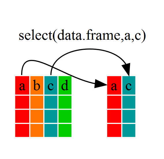
Challenge 1

Write a single command (which can span multiple lines and includes pipes) that will produce a dataframe that has the African values for lifeExp, country and year, but not for other Continents. How many rows does your dataframe have and why?

Solution to Challenge 1

year_country_lifeExp_Africa <- gapminder %>%
                           filter(continent=="Africa") %>%
                           select(year,country,lifeExp)

We can check the number of rows in our new dataframe year_country_lifeExp_Africa by using the ncol command:

nrow(year_country_lifeExp_Africa)

[1] 624

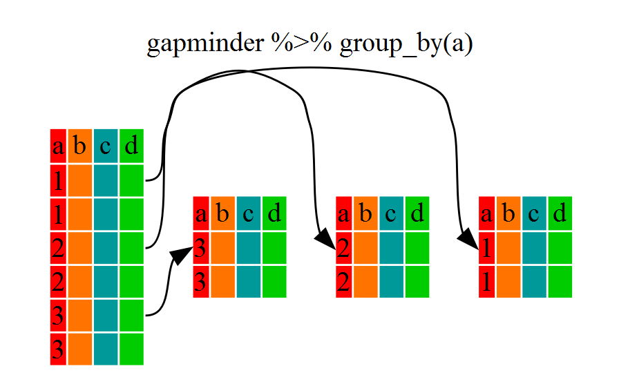
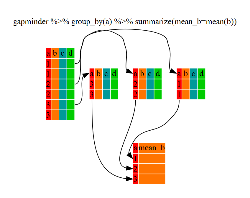
Challenge 2

Calculate the average life expectancy per country. What is the longest average life expectancy and the shortest life expectancy?

Solution to Challenge 2

First let’s build a dataframe with a summary of the average life expectancy per country:

lifeExp_bycountry <- gapminder %>%
   group_by(country) %>%
   summarize(mean_lifeExp=mean(lifeExp))

Now that we have the data we need, we can use the min and max commands to determine which country had the longest and shortest life expectancy:

min(lifeExp_bycountry$mean_lifeExp)

[1] 36.76917

max(lifeExp_bycountry$mean_lifeExp)

[1] 76.51142

Challenge 3

Calculate the average life expectancy in 2002 for each continent.

Solution to Challenge 3

lifeExp_bycontinents <- gapminder %>%
   filter(year==2002) %>%
   group_by(continent) %>%
   summarize(mean_lifeExp=mean(lifeExp))

Challenge 4 - Advanced

Modify your code from Challenge 3 to randomly select 2 countries from each continent before calculating the average life expectancy and then arrange the continent names in reverse order.

Hint: Use the dplyr functions arrange and sample_n, they have similar syntax to other dplyr functions. Be sure to check out the help documentation for the new functions by typing ?arrange or ?sample_n if you run into difficulties.

Solution to Challenge 4

lifeExp_2countries_bycontinents <- gapminder %>%
   filter(year==2002) %>%
   group_by(continent) %>%
   summarize(mean_lifeExp=mean(lifeExp)) %>%
   sample_n(2) %>%
   arrange(desc(mean_lifeExp))

Creating Publication Quality Graphics

Challenge 1

Our example visualizes how the GDP per capita changes in relationship to life expectancy:

ggplot(data = gapminder, aes(x = gdpPercap, y = lifeExp)) + geom_point()

Modify this example so that the plot visualizes how life expectancy has changed over time:

Hint: the gapminder dataset has a column called “year”, which should appear on the x-axis.

Solution to challenge 1

Modify the example so that the figure visualise how life expectancy has changed over time:

ggplot(data = gapminder, aes(x = year, y = lifeExp)) + geom_point()

Challenge 2

In the previous examples and challenge we’ve used the aes function to tell the scatterplot geom about the x and y locations of each point. Another aesthetic property we can modify is the point color. Modify the code from the previous challenge to color the points by the “continent” column. What trends do you see in the data? Are they what you expected?

Solution to challenge 2

In the previous examples and challenge we’ve used the aes function to tell the scatterplot geom about the x and y locations of each point. Another aesthetic property we can modify is the point color. Modify the code from the previous challenge to color the points by the “continent” column. What trends do you see in the data? Are they what you expected?

ggplot(data = gapminder, aes(x = year, y = lifeExp, color=continent)) +
  geom_point()

Challenge 3

Modify the color and size of the points on the point layer in the previous example.

Hint: do not use the aes function, change this by adding arguments to the correct function.

Solution to Challenge 3

Since we want all the points to be the same and are not making this aesthetic specific to the data, we add this to geom_point to make the change effect all points but not the line.

ggplot(data = gapminder, aes(x = gdpPercap, y = lifeExp)) +
 geom_point(size=3, color="orange") + scale_x_log10() +
 geom_smooth(method="lm", size=1.5)

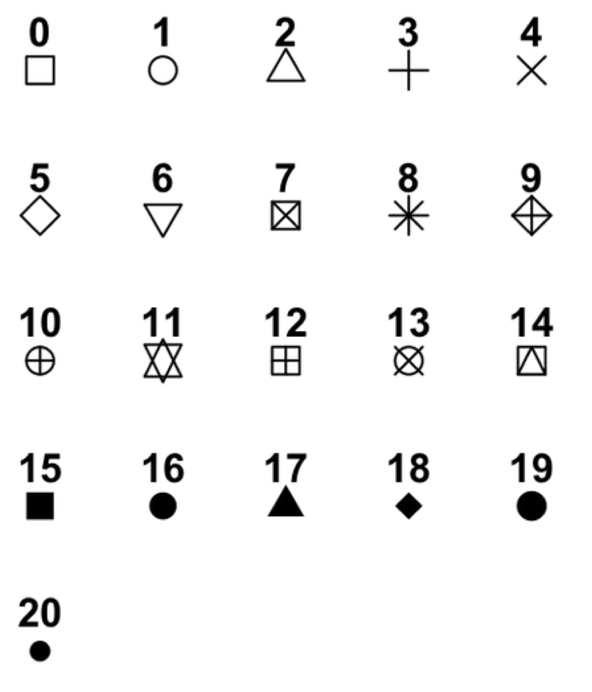
Challenge 4

Modify your solution to Challenge 3 so that the points are now a different shape and are colored by continent with new trendlines.

Hint: The color argument can be used inside the aesthetic. To change the shape of a point, use the pch argument. Setting pch to different numeric values from 1:25 yields different shapes as indicated in the chart below.

Solution to Challenge 4

Since we want the color to be dependent on the continent, we place that argument inside the aes. To change the shape of the point, we place the pch argument inside geom_point.

ggplot(data = gapminder, aes(x = gdpPercap, y = lifeExp, color = continent)) +
geom_point(size=3, pch=17) + scale_x_log10() +
geom_smooth(method="lm", size=1.5)

Challenge 5

Create a density plot of GDP per capita, filled by continent.

Advanced Challenge:

• Transform the x axis to better visualise the data spread.
• Add a facet layer to panel the density plots by year.

Solution to Challenge 5

Create a density plot of GDP per capita, filled by continent.

ggplot(data = gapminder, aes(x = gdpPercap, fill=continent)) +
 geom_density(alpha=0.6)

Advanced:

• Transform the x axis to better visualise the data spread.
• Add a facet layer to panel the density plots by year.

ggplot(data = gapminder, aes(x = gdpPercap, fill=continent)) +
 geom_density(alpha=0.6) + facet_wrap( ~ year) + scale_x_log10()

Writing Data

Challenge 1

Rewrite your ‘pdf’ command to print a second page in the pdf, showing a facet plot of the same data with one panel per continent.

Hint: Remember that we used the facet_wrap command previously to create a facet plot.

Solution to challenge 1

You can output a second plot, by adding a second ggplot command with the facet_wrap command before dev.off command.

pdf("Life_Exp_vs_time2.pdf", width=12, height=4)
ggplot(data=gapminder, aes(x=year, y=lifeExp)) +
  geom_point()
ggplot(data=gapminder, aes(x=year, y=lifeExp)) +
  geom_point() + facet_wrap(~ continent)

# don't forget to close your pdf device!
dev.off()

Challenge 2

Write a data-cleaning script file that subsets the gapminder data to include only data points collected since 1990.

Use this script to write out the new subset to a file your working directory.

Remember to use a different file name so that the new output doesn’t overwrite your old output

Solution to challenge 2

new_data <- gapminder[gapminder$year >= 1990,]
write.table(new_data,
  file="gapminder-1990.csv",
  sep=",",
  quote=FALSE,
  row.names=FALSE
)

Wrapup

If you want to learn more, check out some of these great resources:

Help Files in R

Don’t forget your R helpfiles and package vignettes which can be accessed by using the ? and vignette commands.

Supplemental Lessons

Additional R topics that we could not cover today.

RStudio cheat sheets

R quick reference guides including today’s handouts and more!

R for Data Science

Hadley Wickham is RStudio’s Chief Data Scientist and developer of the dplyr and ggplot2 packages. R for Data Science is his newest book, and is available here for free.

One R Tip a Day on Twitter

Following One R Tip a Day is a great way to learn new tips and tricks in R.

Twotorials

Twotorials is a compilation of 2 minute youtube videos which highlight a specific topic in R.

Quick R Website

Cookbook for R

Advanced R

For more advanced topics, check out Hadley Wickham’s website based on his book “Advanced R”.